Synthetic Controls: A Powerful Way To Measure Policy Impact

Have you ever wondered if a policy change actually has the intended effect?

A few months ago, I stumbled upon a paper by Meehan & Stephenson (2024) that examined the effects of the name change of the Washington Bullets to the Wizards in 1997. The team owner worried that the “Bullets” name was insensitive due to prevalent gun violence in Washington D.C., potentially being an indirect cause of it, and thought that “Wizards” would be a more appropriate name. In the paper, the authors used a technique called the “Synthetic Control Method” to see if the name change actually caused a decrease in homicides per capita in Washington D.C.

The Synthetic Control Method allowed the authors to construct a “Synthetic Washington D.C.” which modeled the counterfactual; what would have happened if the Bullets had not changed their name. The authors found that there was no statistically significantstatistically significant a result in statistical testing that provides enough evidence to reject the null hypothesis, suggesting that an observed effect is likely not due to chance alone difference between the real-life Washington D.C. and its synthetic counterpart, meaning that there was no evidence that the name change caused any detectable decrease in gun violence. I thought that this method of constructing a “synthetic control” was magical. In statistics class, you learn that in an observational study you can never establish a cause-and-effect relationship, you can only find associations. However, using the synthetic control (and the broader fields of econometrics and causal inference) you can find cause-and-effect relationships in observational data if you specify the correct model.

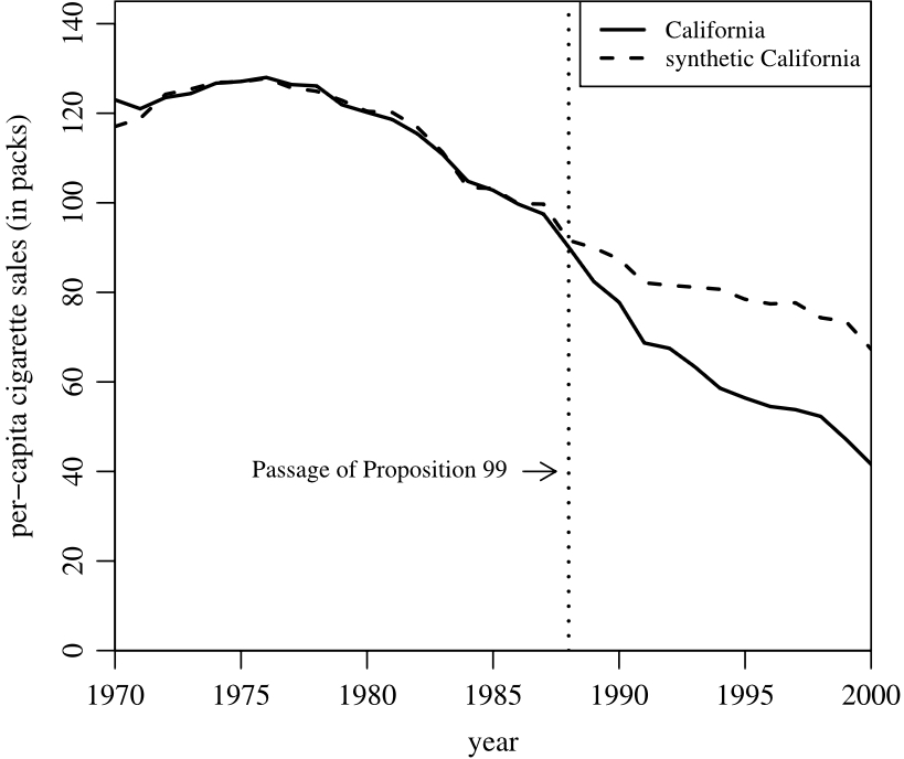
This is especially interesting and important because many policy changes and important questions cannot be properly answered experimentally. This is either because it is unethical to do so (measuring if something causes homicides is obviously unethical), or unfeasible because it is too expensive or difficult to simulate a real world situation in a lab. Since learning about the synthetic control method I have been captivated by it, and also by the broader field of causal inference, the study of finding cause-and-effect through observation. It’s fascinating we can use these methods to quantify the effects of interventions and policies, and answer the crucial question: “What would have occurred if we hadn’t done that?” In one famous example, Abadie et al. (2010) are able to measure the effect of Proposition 99 (cigarette tax) in California on cigarette sales, finding that the tax decreased the per-capita cigarette pack sales by about 26 packs by 2000. This shows that the Proposition 99 accomplished what it set out to do!

How does the synthetic control work?

First, let’s introduce a few key vocabulary words.

• Treatment: The interventionintervention a deliberate action or strategy implemented to produce a desired change or effect in a specific situation or system or condition applied to units in an experiment or study. In the Bullets example, the treatment is the name change.
• Unit: An individual, group, or entity to which a treatment is applied or observed. In the Bullets example, the units are cities.
• Outcome: The variable of interest measured to assess the effect of the treatment. In the Bullets example, the outcome is homicide rate/100k people.
• Counterfactual: The unobserved outcome that represents what would have happened under different treatment conditions. In the Bullets example, this is the hypothetical homicide rate/100k that would have happened if there were no name change.
• Confounder: A variable that is associated with both the treatment and the outcome, potentially leading to a false association between them. For example, one could (falsely) conclude that being taller causes kids to be better at math, even though in reality this is confounded by age: older kids are usually better at math and are also taller.

In a randomized control trial, often considered the “gold-standard” for establishing causality, researchers randomly assign units to either the treatment group or control group. Then they run a statistical test to determine if there is a significant different in outcomes for the treated units compared to the control units. This can establish a cause-and-effect relationship because the assignment of units to either the treatment or control group is completely independent of any of the units’ characteristics; it is randomized. Consequently, the treated group is very likely to closely resemble the untreated group.

With observational data, we don’t have controls. We just know the outcomes of the units and whether or not they were treated. Importantly, we can’t simply compare the outcomes of the treated units to the untreated units; there could be confounders. For example, a city that implements a program to combat homelessness is also likely to be facing high levels of homelessness. It would not be appropriate to compare this city to an untreated city, because that untreated city probably has lower homelessness numbers. So how can we identify units that are similar to our treated unit to act as controls?

This is where the genius of the synthetic control method comes in: we create a new “synthetic control” unit by combining untreated units in a manner that closely approximates our treated unit prior to the treatment. In other words, for a set of untreated units {x₁, x₂, … x_n} and a treated unit x₀, each untreated unit is assigned a weight between 0 and 1. These weights {w₁, w₂, … w_n}, which in total sum to one, are optimized to minimize the difference between x₀ and the weighted sum of units w₁x₁ + w₂x₂+ … + w_nx_n during the pre-treatment period. To enhance the accuracy of the synthetic control, researchers can incorporate additional predictor variables (e.g., population density). This ensures that the synthetic control not only closely mirrors the treated unit in terms of the outcome variable but also approximates it across other relevant metrics. Typically, after optimizing the weights, units significantly dissimilar to the treated unit are assigned a weight of 0, since they do not contribute to the pre-treatment fit. Ultimately, we are left with a combination of units that are very similar to our treated unit.

Below is an example from Abadie et al. (2014) that illustrates how weighing the units in the control group can deliver a significantly better pre-treatment fit than averaging out all of the control units. Notably, in the second image it is much easier to see how Germany diverges compared to its synthetic counterpart, making it clear that West Germany’s GDP per capita dropped as a result of its reunification.

Country	Weight
Austria	0.42
Japan	0.16
Netherlands	0.09
Switzerland	0.11
United States	0.22

How do we measure if the effect of the treatment is statistically significant?

So in the Germany example, we can see that West Germany’s GDP per capita dropped compared to its counterfactual “Synthetic West Germany” after reunification. How can we know that this change is not coincidental, and that reunification actually caused this effect? Firstly, for there to be a significant effect, the post-treatment fit must be poorer than the pre-treatment fit. If the synthetic control closely tracks the treated unit post-treatment, akin to its pre-treatment behavior, it suggests that the treatment may not have had a substantial effect.

Let’s say that our post-treatment fit is worse than our pre-treatment fit. Still, how can we be convinced that this difference is not due to chance? There are many ways to measure whether the treated significantly deviates from the synthetic control. One way is to conduct a “placebo experiment,” where we simulate the synthetic control method for units in the control group, treating each one as if it were the treated unit. By dividing the post-treatment fit by the pre-treatment fit, we can calculate a metric called the mean square prediction error, which quantifies the post-treatment deviation from the counterfactual. Units are then ranked based on this metric, with the expectation that the treated unit will exhibit the highest (or one of the highest) deviations from its synthetic counterpart. In their study on the impact of Proposition 99 on cigarette sales in California, Abadie et al. (2010) employed this method and found that California had the highest mean square prediction error by a significant margin, confirming their finding that Proposition 99 decreased cigarette sales.

Conclusion

In summary, the synthetic control method is a fascinating and powerful way to measure the impact of policies. This blog post is just an introductory glimpse into its potential. Numerous other variations of the synthetic control exist, some using machine learning to improve the pre-treatment fit, and there are new developments every year. Additionally, there are other methods to assess whether the treatment effect is statistically significant or merely coincidental. I hope that this article has piqued your interest and inspires you to read more about the synthetic control method and causal inference. If you are as fascinated by the method and want to know more of the details that go into using the synthetic control, Alberto Abadie (2021), who devised the method, offers a more in-depth description. Adhikari (2021) also provides a thorough and concise guide.

References

Abadie, A. (2021). Using synthetic controls: Feasibility, data requirements, and methodological aspects. Journal of Economic Literature, 59(2), 391–425. https://doi.org/10.1257/jel.20191450

Abadie, A., Diamond, A., & Hainmueller, J. (2010). Synthetic Control Methods for Comparative Case Studies: Estimating the Effect of California’s Tobacco Control Program. Journal of the American Statistical Association, 105(490), 493–505. https://doi.org/10.1198/jasa.2009.ap08746

Abadie, A., Diamond, A., & Hainmueller, J. (2014). Comparative politics and the Synthetic Control Method. American Journal of Political Science, 59(2), 495–510. https://doi.org/10.1111/ajps.12116

Adhikari, B. (2021). A guide to using the synthetic control method to quantify the effects of shocks, policies, and shocking policies. The American Economist, 67(1), 46–63. https://doi.org/10.1177/05694345211019714

Meehan, B., & Stephenson, E. F. (2024). Did the Wizards help Washington Dodge Bullets? Sports Economics Review, 5, 100026. https://doi.org/10.1016/j.serev.2024.100026